Searching & downloading Kepler, K2, and TESS data#
Learning Goals#
By the end of this tutorial, you will:
Understand the data products available to query and download.
Be able to use Lightkurve to search for Kepler/K2 and TESS data products.
Know how to download TESS Full Frame Image cutouts.
Be able to perform a cone search.
Introduction#
The Lightkurve Python package has functions to search for and download observations from Kepler/K2 and TESS. These tools are built to make accessing space telescope data clear and straightforward, with intuitive method and keyword names.
This tutorial outlines what data products are available to query with Lightkurve, and gives examples of how to use the functions to search for and download space telescope observations.
Imports#
This tutorial requires the Lightkurve package, which uses Matplotlib for plotting.
[1]:
%matplotlib inline
import lightkurve as lk
import matplotlib.pyplot as plt
1. What Data Products are Available?#
Kepler/K2 and TESS data products are stored on the Mikulski Archive for Space Telescopes (MAST) in two main forms:
Light curve products: tables containing the measured flux at each observation time.
Target pixel file products: stacks of images with the pixel-level observation at each observation time.
There are also the following additional products available to query and download using Lightkurve:
High Level Science Products (HLSPs): data products produced by a community-created analysis or photometry pipelines. Lightkurve has access to Kepler, K2, and TESS HLSPs. For more information about HLSPs, please see this article on the Space Telescope Science Institute’s archive.
Full Frame Images (FFIs): a file containing all active detector pixels at once. FFIs are currently not available for download through lightkurve, but custom cutouts of TESS FFIs can be queried and downloaded by lightkurve using MAST’s tesscut service.
Lightkurve allows you to query and download each of these data products. The following sections contain examples of how to use the search functions in Lightkurve.
2. Searching for Light Curves#
Lightkurve uses Astroquery to search for data products. Astroquery allows searches based on a target’s coordinates, catalog ID number, or name.
This is passed into the search function using the target keyword, and all valid inputs for identifying a target include:
The name of the object as a string, for example, “Kepler-10.”
The KIC or EPIC identifier as an integer, for example, “11904151.”
A coordinate string in decimal format, for example, “285.67942179 +50.24130576.”
A coordinate string in sexagesimal format, for example, “19:02:43.1 +50:14:28.7.”
An
astropy.coordinates.SkyCoordobject.
You can also specify which mission you would like to retrieve data from using the mission keyword, which takes “Kepler,” “K2,” or “TESS.” By default, all available missions will be returned.
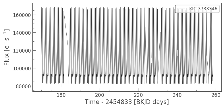
We will start with the case of searching for a Kepler target using its Kepler Input Catalog (KIC) ID number. Below, we search for KIC 3733346, an RR Lyrae star, using the search_lightcurve function.
[2]:
search_result = lk.search_lightcurve('KIC 3733346', author='Kepler')
search_result
[2]:
| # | mission | year | author | exptime | target_name | distance |
|---|---|---|---|---|---|---|
| s | arcsec | |||||
| 0 | Kepler Quarter 01 | 2009 | Kepler | 1800 | kplr003733346 | 0.0 |
| 1 | Kepler Quarter 02 | 2009 | Kepler | 1800 | kplr003733346 | 0.0 |
| 2 | Kepler Quarter 03 | 2009 | Kepler | 1800 | kplr003733346 | 0.0 |
| 3 | Kepler Quarter 04 | 2010 | Kepler | 1800 | kplr003733346 | 0.0 |
| 4 | Kepler Quarter 05 | 2010 | Kepler | 1800 | kplr003733346 | 0.0 |
| 5 | Kepler Quarter 06 | 2010 | Kepler | 1800 | kplr003733346 | 0.0 |
| 6 | Kepler Quarter 07 | 2010 | Kepler | 1800 | kplr003733346 | 0.0 |
| 7 | Kepler Quarter 11 | 2011 | Kepler | 60 | kplr003733346 | 0.0 |
| 8 | Kepler Quarter 08 | 2011 | Kepler | 1800 | kplr003733346 | 0.0 |
| 9 | Kepler Quarter 09 | 2011 | Kepler | 1800 | kplr003733346 | 0.0 |
| 10 | Kepler Quarter 10 | 2011 | Kepler | 1800 | kplr003733346 | 0.0 |
| 11 | Kepler Quarter 11 | 2012 | Kepler | 1800 | kplr003733346 | 0.0 |
| 12 | Kepler Quarter 12 | 2012 | Kepler | 1800 | kplr003733346 | 0.0 |
| 13 | Kepler Quarter 13 | 2012 | Kepler | 1800 | kplr003733346 | 0.0 |
| 14 | Kepler Quarter 14 | 2012 | Kepler | 1800 | kplr003733346 | 0.0 |
| 15 | Kepler Quarter 15 | 2013 | Kepler | 1800 | kplr003733346 | 0.0 |
| 16 | Kepler Quarter 16 | 2013 | Kepler | 1800 | kplr003733346 | 0.0 |
| 17 | Kepler Quarter 17 | 2013 | Kepler | 1800 | kplr003733346 | 0.0 |
search_lightcurve returns a SearchResult table, which contains information about the data products available to download. This search result tells us that KIC 3733346 was observed in Kepler Quarters 1–17.
You can select an individual entry in this search result by indexing the search result.
[3]:
search_result[0]
[3]:
| # | mission | year | author | exptime | target_name | distance |
|---|---|---|---|---|---|---|
| s | arcsec | |||||
| 0 | Kepler Quarter 01 | 2009 | Kepler | 1800 | kplr003733346 | 0.0 |
For more information about the available data products, the SearchResult has a full table accessible by calling .table. This full table contains the columns listed below. Definitions of each of these terms can be found here.
[4]:
for column in search_result.table.columns:
  print(column)
intentType
obs_collection
provenance_name
instrument_name
project
filters
wave_region
target_name
target_classification
obs_id
s_ra
s_dec
dataproduct_type
proposal_pi
calib_level
t_min
t_max
t_exptime
wavelength_region
em_min
em_max
obs_title
t_obs_release
proposal_id
proposal_type
sequence_number
s_region
jpegURL
dataURL
dataRights
mtFlag
srcDen
obsid
objID
wave_min
wave_max
exptime
distance
obsID
obs_collection_products
dataproduct_type_products
description
type
dataURI
productType
productGroupDescription
productSubGroupDescription
productDocumentationURL
project_products
prvversion
proposal_id_products
productFilename
size
parent_obsid
dataRights_products
calib_level_products
filters_products
author
mission
#
year
sort_order
These column names can also be used to search for specific entries in the table.
[5]:
# import numpy, which we will use to find the desired index in the table
import numpy as np
quarter2_index = np.where(search_result.table['mission'] == 'Kepler Quarter 02')[0]
search_result[quarter2_index]
[5]:
| # | mission | year | author | exptime | target_name | distance |
|---|---|---|---|---|---|---|
| s | arcsec | |||||
| 0 | Kepler Quarter 02 | 2009 | Kepler | 1800 | kplr003733346 | 0.0 |
You can also narrow down the list of observations when you make the search using the following mission-specific keywords:
Kepler:
quarterK2:
campaignTESS:
sector
Let’s perform the search for KIC 3733346 again, this time specifying that we only want data from Kepler Quarter 2.
[6]:
search_result_q2 = lk.search_lightcurve('KIC 3733346', author='Kepler', quarter=2)
search_result_q2
[6]:
| # | mission | year | author | exptime | target_name | distance |
|---|---|---|---|---|---|---|
| s | arcsec | |||||
| 0 | Kepler Quarter 02 | 2009 | Kepler | 1800 | kplr003733346 | 0.0 |
2.1 Downloading a single light curve#
A light curve can be downloaded by calling .download().
[7]:
lc = search_result_q2.download()
lc
[7]:
| time | flux | flux_err | quality | timecorr | centroid_col | centroid_row | cadenceno | sap_flux | sap_flux_err | sap_bkg | sap_bkg_err | pdcsap_flux | pdcsap_flux_err | sap_quality | psf_centr1 | psf_centr1_err | psf_centr2 | psf_centr2_err | mom_centr1 | mom_centr1_err | mom_centr2 | mom_centr2_err | pos_corr1 | pos_corr2 |
|---|---|---|---|---|---|---|---|---|---|---|---|---|---|---|---|---|---|---|---|---|---|---|---|---|
| electron / s | electron / s | d | pix | pix | electron / s | electron / s | electron / s | electron / s | electron / s | electron / s | pix | pix | pix | pix | pix | pix | pix | pix | pix | pix | ||||
| Time | float32 | float32 | int32 | float32 | float64 | float64 | int32 | float32 | float32 | float32 | float32 | float32 | float32 | int32 | float64 | float32 | float64 | float32 | float64 | float32 | float64 | float32 | float32 | float32 |
| 169.7659418421681 | 9.2319516e+04 | 9.2697735e+00 | 0 | 3.263322e-03 | 781.81123 | 786.73051 | 2977 | 8.9092305e+04 | 8.8779488e+00 | 2.0773477e+03 | 7.0835429e-01 | 9.2319516e+04 | 9.2697735e+00 | 0 | ——— | ——— | ——— | ——— | 781.81123 | 1.2057812e-04 | 786.73051 | 1.4581889e-04 | 1.0092091e-01 | -1.9298431e-01 |
| 169.7863760557957 | 8.9214008e+04 | 9.1563263e+00 | 0 | 3.263836e-03 | 781.80745 | 786.73005 | 2978 | 8.6126133e+04 | 8.7672691e+00 | 2.0793108e+03 | 7.0831001e-01 | 8.9214008e+04 | 9.1563263e+00 | 0 | ——— | ——— | ——— | ——— | 781.80745 | 1.2411721e-04 | 786.73005 | 1.5003627e-04 | 1.0036582e-01 | -1.9279599e-01 |
| 169.80681006918894 | 8.5608195e+04 | 9.0206089e+00 | 0 | 3.264349e-03 | 781.80376 | 786.72918 | 2979 | 8.2681344e+04 | 8.6362791e+00 | 2.0772085e+03 | 7.0797533e-01 | 8.5608195e+04 | 9.0206089e+00 | 0 | ——— | ——— | ——— | ——— | 781.80376 | 1.2850568e-04 | 786.72918 | 1.5526263e-04 | 1.0042009e-01 | -1.9289577e-01 |
| 169.8272442823436 | 8.3063625e+04 | 8.9255180e+00 | 0 | 3.264862e-03 | 781.80081 | 786.72913 | 2980 | 8.0246992e+04 | 8.5434341e+00 | 2.0767546e+03 | 7.0811391e-01 | 8.3063625e+04 | 8.9255180e+00 | 0 | ——— | ——— | ——— | ——— | 781.80081 | 1.3182692e-04 | 786.72913 | 1.5920549e-04 | 1.0021163e-01 | -1.9266903e-01 |
| 169.84767829527118 | 8.4244992e+04 | 8.9700022e+00 | 0 | 3.265375e-03 | 781.80242 | 786.72905 | 2981 | 8.1373969e+04 | 8.5879698e+00 | 2.0805510e+03 | 7.0775980e-01 | 8.4244992e+04 | 8.9700022e+00 | 0 | ——— | ——— | ——— | ——— | 781.80242 | 1.3028238e-04 | 786.72905 | 1.5737538e-04 | 1.0010726e-01 | -1.9241102e-01 |
| 169.86811250773462 | 9.7360805e+04 | 9.4567146e+00 | 0 | 3.265888e-03 | 781.81441 | 786.73210 | 2982 | 9.3887734e+04 | 9.0560179e+00 | 2.0782170e+03 | 7.0836788e-01 | 9.7360805e+04 | 9.4567146e+00 | 0 | ——— | ——— | ——— | ——— | 781.81441 | 1.1529749e-04 | 786.73210 | 1.3958653e-04 | 9.8970458e-02 | -1.9224431e-01 |
| 169.88854651995644 | 1.2825345e+05 | 1.0503614e+01 | 0 | 3.266400e-03 | 781.83651 | 786.73500 | 2983 | 1.2337022e+05 | 1.0063412e+01 | 2.0774846e+03 | 7.0743954e-01 | 1.2825345e+05 | 1.0503614e+01 | 0 | ——— | ——— | ——— | ——— | 781.83651 | 9.1639682e-05 | 786.73500 | 1.1152634e-04 | 9.9608414e-02 | -1.9224758e-01 |
| 169.90898063195345 | 1.5187158e+05 | 1.1233888e+01 | 0 | 3.266912e-03 | 781.84701 | 786.73606 | 2984 | 1.4590969e+05 | 1.0766508e+01 | 2.0792261e+03 | 7.0833290e-01 | 1.5187158e+05 | 1.1233888e+01 | 0 | ——— | ——— | ——— | ——— | 781.84701 | 7.9801415e-05 | 786.73606 | 9.7487238e-05 | 9.8825477e-02 | -1.9200189e-01 |
| 169.9294148437184 | 1.6871948e+05 | 1.1725034e+01 | 0 | 3.267424e-03 | 781.85356 | 786.73615 | 2985 | 1.6198620e+05 | 1.1240104e+01 | 2.0780894e+03 | 7.0873052e-01 | 1.6871948e+05 | 1.1725034e+01 | 0 | ——— | ——— | ——— | ——— | 781.85356 | 7.3274212e-05 | 786.73615 | 8.9778732e-05 | 9.9280514e-02 | -1.9207963e-01 |
| ... | ... | ... | ... | ... | ... | ... | ... | ... | ... | ... | ... | ... | ... | ... | ... | ... | ... | ... | ... | ... | ... | ... | ... | ... |
| 258.28361569694243 | 9.2878820e+04 | 9.2731094e+00 | 0 | 2.597577e-03 | 781.66157 | 787.06740 | 7309 | 8.8527227e+04 | 8.8611145e+00 | 2.1467869e+03 | 7.0827138e-01 | 9.2878820e+04 | 9.2731094e+00 | 0 | ——— | ——— | ——— | ——— | 781.66157 | 1.2219569e-04 | 787.06740 | 1.4442031e-04 | -5.1394299e-02 | 1.4658417e-01 |
| 258.3040484127632 | 9.2034094e+04 | 9.2417078e+00 | 1100000000000000000 | 2.596793e-03 | 781.65987 | 787.06772 | 7310 | 8.7705906e+04 | 8.8319845e+00 | 2.1418911e+03 | 7.0921260e-01 | 9.2034094e+04 | 9.2417078e+00 | 1100000000000000000 | ——— | ——— | ——— | ——— | 781.65987 | 1.2317530e-04 | 787.06772 | 1.4557109e-04 | -5.2788489e-02 | 1.4718631e-01 |
| 258.32448132812715 | 9.1409266e+04 | 9.2205820e+00 | 0 | 2.596008e-03 | 781.66046 | 787.06774 | 7311 | 8.7112359e+04 | 8.8111296e+00 | 2.1419580e+03 | 7.0941931e-01 | 9.1409266e+04 | 9.2205820e+00 | 0 | ——— | ——— | ——— | ——— | 781.66046 | 1.2387938e-04 | 787.06774 | 1.4640002e-04 | -5.1082097e-02 | 1.4737232e-01 |
| 258.34491414348304 | 9.0934453e+04 | 9.2037315e+00 | 0 | 2.595223e-03 | 781.66006 | 787.06733 | 7312 | 8.6663805e+04 | 8.7947636e+00 | 2.1399746e+03 | 7.0873111e-01 | 9.0934453e+04 | 9.2037315e+00 | 0 | ——— | ——— | ——— | ——— | 781.66006 | 1.2442317e-04 | 787.06733 | 1.4701700e-04 | -5.1297914e-02 | 1.4743482e-01 |
| 258.3653468583798 | 9.0627711e+04 | 9.1926651e+00 | 0 | 2.594438e-03 | 781.65842 | 787.06748 | 7313 | 8.6410219e+04 | 8.7850523e+00 | 2.1412927e+03 | 7.0846963e-01 | 9.0627711e+04 | 9.1926651e+00 | 0 | ——— | ——— | ——— | ——— | 781.65842 | 1.2473276e-04 | 787.06748 | 1.4736662e-04 | -5.3477854e-02 | 1.4825350e-01 |
| 258.4062125879427 | 9.2799812e+04 | 9.2735319e+00 | 0 | 2.592868e-03 | 781.66311 | 787.06602 | 7315 | 8.8482406e+04 | 8.8615150e+00 | 2.1397761e+03 | 7.0821041e-01 | 9.2799812e+04 | 9.2735319e+00 | 0 | ——— | ——— | ——— | ——— | 781.66311 | 1.2222759e-04 | 787.06602 | 1.4448226e-04 | -5.0823554e-02 | 1.4643176e-01 |
| 258.4266453021337 | 9.2305727e+04 | 9.2546864e+00 | 0 | 2.592082e-03 | 781.66219 | 787.06568 | 7316 | 8.8041828e+04 | 8.8437214e+00 | 2.1407056e+03 | 7.0872313e-01 | 9.2305727e+04 | 9.2546864e+00 | 0 | ——— | ——— | ——— | ——— | 781.66219 | 1.2274201e-04 | 787.06568 | 1.4511198e-04 | -5.2071981e-02 | 1.4703403e-01 |
| 258.4470781163327 | 8.9541500e+04 | 9.1516228e+00 | 0 | 2.591296e-03 | 781.65845 | 787.06562 | 7317 | 8.5375305e+04 | 8.7458200e+00 | 2.1410559e+03 | 7.0890176e-01 | 8.9541500e+04 | 9.1516228e+00 | 0 | ——— | ——— | ——— | ——— | 781.65845 | 1.2598942e-04 | 787.06562 | 1.4883128e-04 | -5.3206120e-02 | 1.4745203e-01 |
| 258.46751103029237 | 8.5948555e+04 | 9.0121727e+00 | 0 | 2.590510e-03 | 781.65486 | 787.06465 | 7318 | 8.1906250e+04 | 8.6120892e+00 | 2.1406807e+03 | 7.0841718e-01 | 8.5948555e+04 | 9.0121727e+00 | 0 | ——— | ——— | ——— | ——— | 781.65486 | 1.3045572e-04 | 787.06465 | 1.5403067e-04 | -5.2536737e-02 | 1.4800853e-01 |
This returns a single KeplerLightCurve object, which is shown above in the form of an astropy table. We can examine the light curve using the plot method.
[8]:
lc.plot();
2.2 Downloading a collection of light curves#
The SearchResult object also has a download_all method, allowing you to download multiple light curves. This returns a LightCurveCollection, a convenient container for LightCurve objects.
[9]:
lc_collection = search_result[:5].download_all()
lc_collection
[9]:
LightCurveCollection of 5 objects:
    0: <KeplerLightCurve LABEL="KIC 3733346" QUARTER=1 AUTHOR=Kepler FLUX_ORIGIN=pdcsap_flux>
    1: <KeplerLightCurve LABEL="KIC 3733346" QUARTER=2 AUTHOR=Kepler FLUX_ORIGIN=pdcsap_flux>
    2: <KeplerLightCurve LABEL="KIC 3733346" QUARTER=3 AUTHOR=Kepler FLUX_ORIGIN=pdcsap_flux>
    3: <KeplerLightCurve LABEL="KIC 3733346" QUARTER=4 AUTHOR=Kepler FLUX_ORIGIN=pdcsap_flux>
    4: <KeplerLightCurve LABEL="KIC 3733346" QUARTER=5 AUTHOR=Kepler FLUX_ORIGIN=pdcsap_flux>
The LightCurveCollection has a number of useful functions for plotting and manipulating the light curves. For more information about how to combine multiple light curves, please see the tutorial on combining multiple quarters of Kepler observations.
One of the methods the collection enables you to use is plot, making it possible to quickly visualize all observations in your collection.
[10]:
# Create a larger figure for clarity
fig, ax = plt.subplots(figsize=(20,5))
# Plot the light curve collection
lc_collection.plot(ax=ax);

You can also iterate through a collection to label them more clearly and to perform additional actions like normalization.
[11]:
fig, ax = plt.subplots(figsize=(20,5))
for lc in lc_collection:
  lc.normalize().plot(ax=ax, label=f'Quarter {lc.quarter}');

3. Searching for Target Pixel Files#
The other primary data product used by Lightkurve is the TargetPixelFile, or TPF. A TPF is a stack of images containing the flux in each pixel at each cadence.
Similar to the approach above, we can use the search_targetpixelfile method to identify available observations.
[12]:
search_result = lk.search_targetpixelfile('K2-199', exptime=1800)
search_result
[12]:
This returns a table which contains the same information as a light curve search result.
3.1 Downloading a single target pixel file#
When you call download on a search result containing more than one entry, it will download only the first entry in the search result. Lightkurve will raise a friendly warning to let you know when this occurs.
[13]:
tpf = search_result.download()
/Users/tapritc2/tessgi/dev/lightkurve/lkmain-docs/lightkurve/src/lightkurve/search.py:421: LightkurveWarning: Warning: 2 files available to download. Only the first file has been downloaded. Please use `download_all()` or specify additional criteria (e.g. quarter, campaign, or sector) to limit your search.
  warnings.warn(
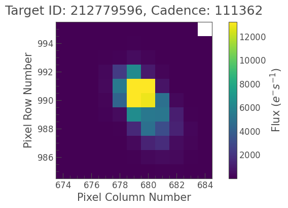
We can view a single cadence of the TPF using the plot method.
[14]:
tpf.plot();
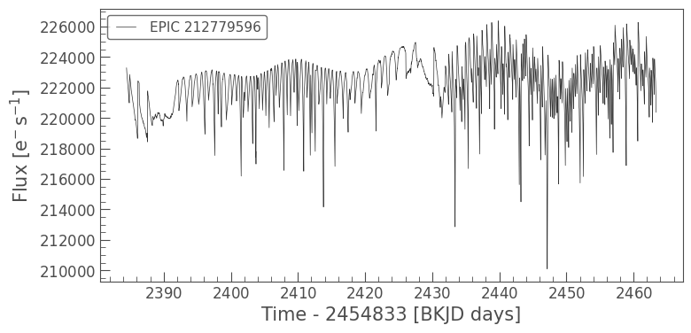
If we want to turn the TPF into a light curve, there is a to_lightcurve method.
[15]:
lc = tpf.to_lightcurve()
lc.plot();
For more information about using and plotting TPFs, please see the tutorials on using Kepler target pixel file products with Lightkurve and plotting Kepler target pixel file products with Lightkurve.
3.2 Downloading a collection of target pixel files#
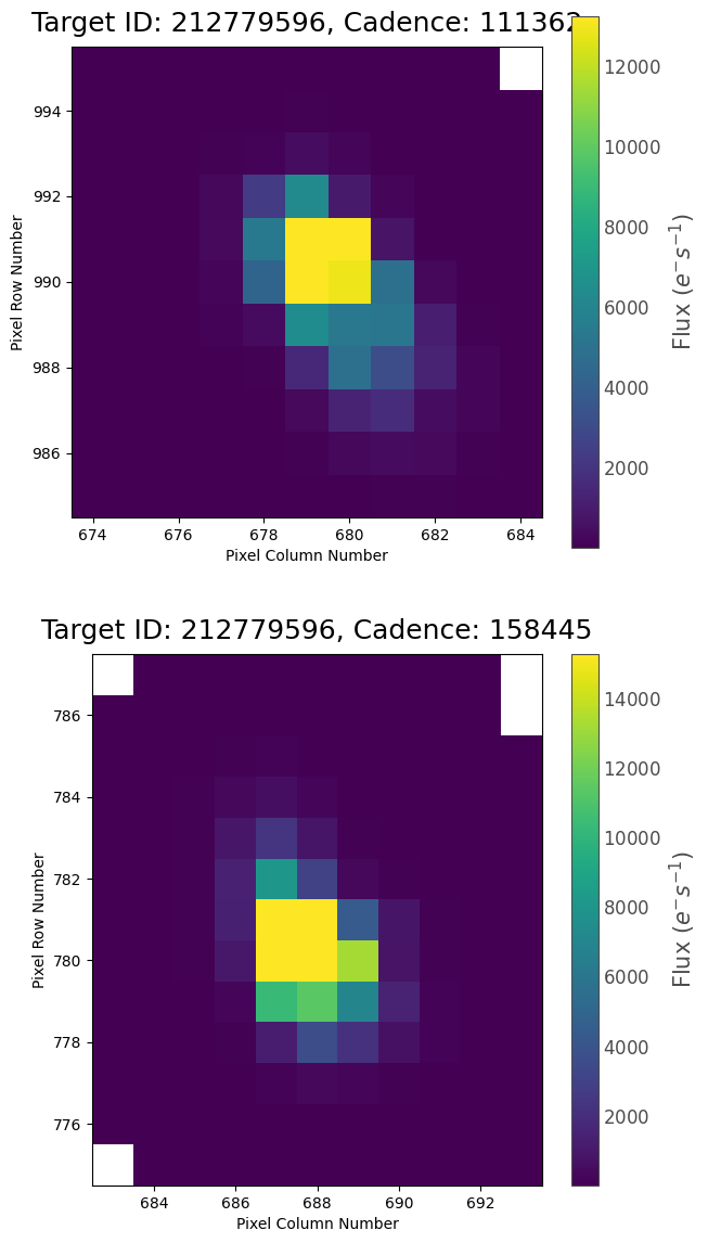
As with the lightcurve collection introduced in Section 2.2, you can also download multiple TPFs at a time using the download_all method, which returns a TargetPixelFileCollection.
[16]:
tpf_collection = search_result.download_all()
tpf_collection
[16]:
TargetPixelFileCollection of 2 objects:
    0: KeplerTargetPixelFile Object (ID: 212779596)
    1: KeplerTargetPixelFile Object (ID: 212779596)
A single cadence of each of these TPFs can be inspected with the plot method.
[17]:
tpf_collection.plot();
4. Searching for TESS Full Frame Image (FFI) Cutouts#
It is also possible to download targets observed in the TESS Full Frame Images (FFIs) using Lightkurve. This is done using search_tesscut, which utilizes the TESSCut tool (Brasseur et. al 2019).
[18]:
search_result = lk.search_tesscut('Pi Men')
search_result
[18]:
| # | mission | year | author | exptime | target_name | distance |
|---|---|---|---|---|---|---|
| s | arcsec | |||||
| 0 | TESS Sector 04 | 2018 | TESScut | 1426 | Pi Men | 0.0 |
| 1 | TESS Sector 01 | 2018 | TESScut | 1426 | Pi Men | 0.0 |
| 2 | TESS Sector 13 | 2019 | TESScut | 1426 | Pi Men | 0.0 |
| 3 | TESS Sector 11 | 2019 | TESScut | 1426 | Pi Men | 0.0 |
| 4 | TESS Sector 12 | 2019 | TESScut | 1426 | Pi Men | 0.0 |
| 5 | TESS Sector 08 | 2019 | TESScut | 1426 | Pi Men | 0.0 |
| 6 | TESS Sector 27 | 2020 | TESScut | 475 | Pi Men | 0.0 |
| 7 | TESS Sector 31 | 2020 | TESScut | 475 | Pi Men | 0.0 |
| 8 | TESS Sector 28 | 2020 | TESScut | 475 | Pi Men | 0.0 |
| 9 | TESS Sector 39 | 2021 | TESScut | 475 | Pi Men | 0.0 |
| 10 | TESS Sector 38 | 2021 | TESScut | 475 | Pi Men | 0.0 |
| 11 | TESS Sector 34 | 2021 | TESScut | 475 | Pi Men | 0.0 |
| 12 | TESS Sector 35 | 2021 | TESScut | 475 | Pi Men | 0.0 |
| 13 | TESS Sector 68 | 2023 | TESScut | 158 | Pi Men | 0.0 |
| 14 | TESS Sector 61 | 2023 | TESScut | 158 | Pi Men | 0.0 |
| 15 | TESS Sector 65 | 2023 | TESScut | 158 | Pi Men | 0.0 |
| 16 | TESS Sector 66 | 2023 | TESScut | 158 | Pi Men | 0.0 |
| 17 | TESS Sector 67 | 2023 | TESScut | 158 | Pi Men | 0.0 |
| 18 | TESS Sector 62 | 2023 | TESScut | 158 | Pi Men | 0.0 |
| 19 | TESS Sector 64 | 2023 | TESScut | 158 | Pi Men | 0.0 |
| 20 | TESS Sector 93 | 2025 | TESScut | 158 | Pi Men | 0.0 |
| 21 | TESS Sector 94 | 2025 | TESScut | 158 | Pi Men | 0.0 |
| 22 | TESS Sector 95 | 2025 | TESScut | 158 | Pi Men | 0.0 |
| 23 | TESS Sector 88 | 2025 | TESScut | 158 | Pi Men | 0.0 |
| 24 | TESS Sector 89 | 2025 | TESScut | 158 | Pi Men | 0.0 |
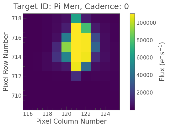
TESS FFI cutouts are downloaded as TargetPixelFile objects. This is done using the same download function as above, but it now takes an additional argument cutout_size, which describes the number of pixels along the side of the cutout, and can be an int or a tuple.
[19]:
tpf_cutout = search_result[0].download(cutout_size=10)
tpf_cutout.plot();
5. Performing a Cone Search#
If you are interested in identifying a number of nearby targets, you can perform a cone search, which will return all available targets within a cone of a specfied radius on the sky. The radius can be either a float or an astropy.units.Quantity object. If a float is given, it will be assumed to be in units of arcseconds. If None then we default to 0.0001 arcsec.
[20]:
search_result = lk.search_targetpixelfile('Trappist-1', radius=180., campaign=12, exptime=1800)
print(search_result)
SearchResult containing 3 data products.

 #     mission     year author exptime  target_name  distance
                                  s                   arcsec
--- -------------- ---- ------ ------- ------------- --------
  0 K2 Campaign 12 2016     K2    1800 ktwo246199087      0.0
  1 K2 Campaign 12 2016     K2    1800 ktwo200164267     12.1
  2 K2 Campaign 12 2016     K2    1800 ktwo246199173     95.5
The distance column describes the distance on the sky in arcseconds from the target or coordinates passed into the search.
About this Notebook#
Authors: Nicholas Saunders (nksaun@hawaii.edu)
Updated: September 28, 2020
Citing Lightkurve and Astropy#
If you use lightkurve or its dependencies in your published research, please cite the authors. Click the buttons below to copy BibTeX entries to your clipboard.
[21]:
lk.show_citation_instructions()
[21]:
When using Lightkurve, we kindly request that you cite the following packages:
- lightkurve
- astropy
- astroquery — if you are using search_lightcurve() or search_targetpixelfile().
- tesscut — if you are using search_tesscut().


