Using Light Curve Files with Lightkurve#

Learning Goals#

By the end of this tutorial, you will:

Understand how NASA’s Kepler Mission collected and released light curve data products.
Be able to download and plot light curve files from the data archive using Lightkurve.
Be able to access light curve metadata.
Understand the time and brightness units.

Introduction#

The Kepler, K2, and TESS telescopes observe stars for long periods of time, from just under a month to four years. By doing so they observe how the brightness of stars change over time. A series of these brightness observations is referred to as a light curve of a star.

Light curves of stars observed by the Kepler, K2, or TESS missions are created from the raw images collected by these telescopes using software built for this purpose by the mission teams. In this tutorial, we will learn how to use the Lightkurve package to download these preprocessed light curves from Kepler’s data archive, plot them, and understand their properties and units.

Much of the explanation below is inspired by Kinemuchi et al. (2012), an excellent paper introducing and explaining the terminology surrounding the Kepler mission and its data. You can find detailed information on the mission and its data products in the official Kepler Instrument Handbook and the Kepler Data Processing Handbook.

We will use the Kepler mission as the main example, but these tools are extensible to TESS and K2 as well. For example, while in this tutorial we will learn to work with Lightkurve’s KeplerLightCurve objects, there are also TessLightCurve objects that work in the same way.

Imports#

This tutorial only requires the Lightkurve package, which in turn uses matplotlib for plotting.

[1]:

import lightkurve as lk
%matplotlib inline

1. About NASA’s Photometric Space Telescopes#

In order to understand the data produced by NASA’s Kepler, K2, and TESS missions, it is useful to understand a little about how these data were obtained.

1.1. Kepler #

During its nominal mission, the Kepler telescope made observations using 21 pairs of rectangular charge-coupled device (CCD) camera chips (also called modules), each consisting of four 1100 x 2048 pixel channels. Each observed star fell on one of these 84 CCD channels. Recording the channel numbers for each star was important, because the Kepler spacecraft rotated by 90 degrees roughly four times a year. These rotations divide what are referred to as observing quarters. While the same star may be observed in multiple quarters, it may fall on a different CCD channel each time.

Kepler observed a single field in the sky, although not all stars in this field were recorded as light curves. Instead, pixels were selected around a predetermined list of target stars, which were then downloaded. These downloaded measurements are stored in target pixel files (TPFs). By adding up the flux (a measurement of an object’s brightness per unit time) measured by the pixels in which a target star appears, the total brightness of a star can be measured. If you make this measurement at different times, you obtain a light curve.

Kepler recorded the brightness measurements at two different cadences: a Short Cadence (SC, 58.85 seconds) and a Long Cadence (LC, 29.4 minutes). For more details, read: Kepler Instrument Handbook, Section 2.1. Mission Overview and 2.6. Pixels of Interest, and the Kepler Archive Manual Chapter 2: Kepler Data Products.

bf1bc9153e244d709ee125fc535f9fb9

Figure: The field of view of the Kepler mission. The rectangles represent the CCD modules described above.

1.2. K2 #

The Kepler mission ended in 2013 following the loss of two reaction wheels, leaving the spacecraft unable to stay fixed on one portion of the sky. Instead, it changed its focus to the ecliptic plane, and performed 80-day observing campaigns of 19 separate fields. K2 data are very similar to Kepler data, but are subject to higher levels of instrument noise due to the increased instability of the spacecraft. For more details read the K2 Handbook, specifically Section 2: What’s New in K2.

1.3. TESS #

The Transiting Exoplanet Survey Satellite (TESS) succeeded Kepler in 2018. The data it collects are very similar to those from Kepler and K2, but TESS covers a much larger area of the sky at a lower resolution. TESS observes large sectors of the sky for 27 days at a time. The overlap of these sectors means that stars near the ecliptic poles will receive a year of uninterrupted data, while those near the ecliptic receive only ~27 days. Compared to Kepler, TESS observes in several different cadence modes, including 20 seconds, 120 seconds, 10 minutes, and 30 minutes. For more details, see the Mission Overview and the TESS Instrument Handbook, specifically Section 2: Introduction to TESS.

Some stars that have been observed by TESS will also have been observed by Kepler, and in some rare cases K2.

2. Downloading a Light Curve File#

The light curves of stars created by the Kepler mission are stored at the Mikulksi Archive for Space Telescopes (MAST) archive, along with metadata about the observations, such as which CCD channel was used at each time.

Lightkurve’s built-in tools allow us to search for light curve files in the archive, and download them and their metadata. In this example, we will start by downloading one quarter of Kepler data for a star named Kepler-8, a star somewhat larger than the Sun, and the host of a hot Jupiter planet.

Using Lightkurve’s search_lightcurve function, we can find an itemized list of different light curve file products available for Kepler-8:

[2]:

search_result = lk.search_lightcurve("Kepler-8", author="Kepler", cadence="long")
search_result

[2]:

SearchResult containing 18 data products.

#	mission	year	author	exptime	target_name	distance
				s		arcsec
0	Kepler Quarter 00	2009	Kepler	1800	kplr006922244	0.0
1	Kepler Quarter 01	2009	Kepler	1800	kplr006922244	0.0
2	Kepler Quarter 02	2009	Kepler	1800	kplr006922244	0.0
3	Kepler Quarter 03	2009	Kepler	1800	kplr006922244	0.0
4	Kepler Quarter 04	2010	Kepler	1800	kplr006922244	0.0
5	Kepler Quarter 05	2010	Kepler	1800	kplr006922244	0.0
6	Kepler Quarter 06	2010	Kepler	1800	kplr006922244	0.0
7	Kepler Quarter 07	2010	Kepler	1800	kplr006922244	0.0
8	Kepler Quarter 10	2011	Kepler	1800	kplr006922244	0.0
9	Kepler Quarter 08	2011	Kepler	1800	kplr006922244	0.0
10	Kepler Quarter 09	2011	Kepler	1800	kplr006922244	0.0
11	Kepler Quarter 11	2012	Kepler	1800	kplr006922244	0.0
12	Kepler Quarter 12	2012	Kepler	1800	kplr006922244	0.0
13	Kepler Quarter 13	2012	Kepler	1800	kplr006922244	0.0
14	Kepler Quarter 14	2012	Kepler	1800	kplr006922244	0.0
15	Kepler Quarter 16	2013	Kepler	1800	kplr006922244	0.0
16	Kepler Quarter 15	2013	Kepler	1800	kplr006922244	0.0
17	Kepler Quarter 17	2013	Kepler	1800	kplr006922244	0.0

In this list, each row represents a different observing period. We find that Kepler recorded the maxmimum of 18 quarters of data for this target across four years. The observation column lists the Kepler Quarter. The target_name represents the Kepler Input Catalogue (KIC) ID of the target, and the productFilename column is the name of the FITS files downloaded from MAST. The distance column shows the separation on the sky between the searched coordinates and the downloaded objects — this is only relevant when you pass a radius argument to the search_lightcurve function to search for targets within a given search radius around a set of coordinates.

The search_lightcurve function takes several additional arguments, such as the quarter number or the mission name.

The search function returns a SearchResult object which has several convenient operations. For example, we can select the fourth data product in the list as follows:

[3]:

search_result[4]

[3]:

SearchResult containing 1 data products.

#	mission	year	author	exptime	target_name	distance
				s		arcsec
0	Kepler Quarter 04	2010	Kepler	1800	kplr006922244	0.0

We can download this data product using the download() method:

[4]:

klc = search_result[4].download()

This instruction is identical to the following line:

[5]:

klc = lk.search_lightcurve("Kepler-8", author="Kepler", cadence="long", quarter=4).download()

The klc variable we have obtained in this way is a KeplerLightCurve object. This object contains time, flux, and flux error information, as well as a whole lot of data about spacecraft systematics. We can view all of them by calling the object by itself:

[6]:

klc

[6]:

KeplerLightCurve length=4116 LABEL="KIC 6922244" QUARTER=4 AUTHOR=Kepler FLUX_ORIGIN=pdcsap_flux

time	flux	flux_err	quality	timecorr	centroid_col	centroid_row	cadenceno	sap_flux	sap_flux_err	sap_bkg	sap_bkg_err	pdcsap_flux	pdcsap_flux_err	sap_quality	psf_centr1	psf_centr1_err	psf_centr2	psf_centr2_err	mom_centr1	mom_centr1_err	mom_centr2	mom_centr2_err	pos_corr1	pos_corr2
	electron / s	electron / s		d	pix	pix		electron / s	electron / s	electron / s	electron / s	electron / s	electron / s		pix	pix	pix	pix	pix	pix	pix	pix	pix	pix
Time	float32	float32	int32	float32	float64	float64	int32	float32	float32	float32	float32	float32	float32	int32	float64	float32	float64	float32	float64	float32	float64	float32	float32	float32
352.37632485035283	———	———	0	-1.410670e-03	682.69125	190.13296	11914	4.3689148e+04	6.6459765e+00	1.6722699e+03	4.6767941e-01	———	———	0	682.60927	7.8001787e-05	190.36814	1.1752916e-04	682.69125	1.8638317e-04	190.13296	1.8306405e-04	9.8764673e-02	-1.7217098e-01
352.3967580484896	5.2490750e+04	8.0003128e+00	10000000000000	-1.411072e-03	682.69084	190.13270	11915	4.3698070e+04	6.6462421e+00	1.6698400e+03	4.6764868e-01	5.2490750e+04	8.0003128e+00	10000000000000	682.60900	7.7997785e-05	190.36777	1.1751152e-04	682.69084	1.8633612e-04	190.13270	1.8303936e-04	9.8700106e-02	-1.7229939e-01
352.4376244455707	5.2484055e+04	7.9999790e+00	10000	-1.411874e-03	682.69038	190.13302	11917	4.3694105e+04	6.6461620e+00	1.6731306e+03	4.6705514e-01	5.2484055e+04	7.9999790e+00	10000	682.60862	7.7994831e-05	190.36848	1.1754913e-04	682.69038	1.8634219e-04	190.13302	1.8301954e-04	9.8306537e-02	-1.7180158e-01
352.45805764463876	5.2491809e+04	8.0006199e+00	0	-1.412275e-03	682.69084	190.13257	11918	4.3698316e+04	6.6463132e+00	1.6741406e+03	4.6687824e-01	5.2491809e+04	8.0006199e+00	0	682.60872	7.7998680e-05	190.36792	1.1751390e-04	682.69084	1.8635279e-04	190.13257	1.8304381e-04	9.8410256e-02	-1.7202987e-01
352.4784908439324	5.2478277e+04	7.9992733e+00	0	-1.412676e-03	682.68949	190.13304	11919	4.3687648e+04	6.6459165e+00	1.6723815e+03	4.6764576e-01	5.2478277e+04	7.9992733e+00	0	682.60829	7.7993544e-05	190.36814	1.1756293e-04	682.68949	1.8641398e-04	190.13304	1.8308057e-04	9.8039381e-02	-1.7183834e-01
352.4989240434661	5.2475855e+04	7.9986620e+00	0	-1.413077e-03	682.69036	190.13318	11920	4.3686480e+04	6.6458707e+00	1.6734375e+03	4.6817183e-01	5.2475855e+04	7.9986620e+00	0	682.60852	7.7998702e-05	190.36875	1.1761812e-04	682.69036	1.8637831e-04	190.13318	1.8304847e-04	9.8102726e-02	-1.7151666e-01
352.5193572433491	5.2487070e+04	7.9990516e+00	0	-1.413477e-03	682.69073	190.13307	11921	4.3692590e+04	6.6460714e+00	1.6731461e+03	4.6760359e-01	5.2487070e+04	7.9990516e+00	0	682.60880	7.8005593e-05	190.36825	1.1757523e-04	682.69073	1.8636670e-04	190.13307	1.8304495e-04	9.8343305e-02	-1.7184900e-01
352.53979034345684	5.2507734e+04	8.0051088e+00	10000000	-1.413877e-03	682.68909	190.13338	11922	4.3712012e+04	6.6500912e+00	1.6725844e+03	4.6755314e-01	5.2507734e+04	8.0051088e+00	10000000	682.60829	7.7979123e-05	190.36859	1.1755893e-04	682.68909	1.8644832e-04	190.13338	1.8299681e-04	9.8101854e-02	-1.7161448e-01
352.56022364380624	5.2472902e+04	8.0007839e+00	0	-1.414276e-03	682.69022	190.13343	11923	4.3683984e+04	6.6457977e+00	1.6750397e+03	4.6755785e-01	5.2472902e+04	8.0007839e+00	0	682.60824	7.7997676e-05	190.36889	1.1760603e-04	682.69022	1.8638840e-04	190.13343	1.8307337e-04	9.7997010e-02	-1.7128757e-01
352.5806568445041	5.2490586e+04	8.0011005e+00	0	-1.414675e-03	682.69067	190.13353	11924	4.3696762e+04	6.6464057e+00	1.6747676e+03	4.6741170e-01	5.2490586e+04	8.0011005e+00	0	682.60858	7.7987701e-05	190.36867	1.1758389e-04	682.69067	1.8633297e-04	190.13353	1.8302842e-04	9.8154068e-02	-1.7160916e-01
352.6010899455432	5.2484711e+04	8.0012350e+00	0	-1.415074e-03	682.69027	190.13306	11925	4.3693148e+04	6.6461196e+00	1.6724357e+03	4.6762615e-01	5.2484711e+04	8.0012350e+00	0	682.60849	7.7995923e-05	190.36871	1.1761376e-04	682.69027	1.8637281e-04	190.13306	1.8304559e-04	9.8116107e-02	-1.7139660e-01
352.6215232468239	5.2479773e+04	8.0013390e+00	10000000000000	-1.415473e-03	682.69014	190.13359	11926	4.3691348e+04	6.6462650e+00	1.6751807e+03	4.6757978e-01	5.2479773e+04	8.0013390e+00	10000000000000	682.60795	7.7985074e-05	190.36936	1.1769431e-04	682.69014	1.8639400e-04	190.13359	1.8310899e-04	9.7724356e-02	-1.7103195e-01
352.64195644845313	5.2499305e+04	8.0007114e+00	0	-1.415872e-03	682.69019	190.13330	11927	4.3703137e+04	6.6466208e+00	1.6736156e+03	4.6751177e-01	5.2499305e+04	8.0007114e+00	0	682.60841	7.7987228e-05	190.36887	1.1764505e-04	682.69019	1.8633960e-04	190.13330	1.8302450e-04	9.8125741e-02	-1.7140007e-01
352.6623896503079	5.2484117e+04	8.0014248e+00	0	-1.416270e-03	682.69002	190.13337	11928	4.3692902e+04	6.6462936e+00	1.6730603e+03	4.6794355e-01	5.2484117e+04	8.0014248e+00	0	682.60814	7.7984361e-05	190.36915	1.1766269e-04	682.69002	1.8636827e-04	190.13337	1.8306459e-04	9.7747400e-02	-1.7097178e-01
352.68282285240275	5.2487891e+04	8.0007782e+00	0	-1.416668e-03	682.68996	190.13380	11929	4.3696273e+04	6.6464286e+00	1.6735245e+03	4.6725965e-01	5.2487891e+04	8.0007782e+00	0	682.60813	7.7983277e-05	190.36919	1.1766609e-04	682.68996	1.8634208e-04	190.13380	1.8304669e-04	9.7714014e-02	-1.7095777e-01
352.70325605484686	5.2454434e+04	7.9984565e+00	0	-1.417065e-03	682.69014	190.13340	11930	4.3666207e+04	6.6449828e+00	1.6736576e+03	4.6680400e-01	5.2454434e+04	7.9984565e+00	0	682.60832	7.8020654e-05	190.36883	1.1766910e-04	682.69014	1.8649764e-04	190.13340	1.8317846e-04	9.7894058e-02	-1.7119597e-01
352.7236892575165	5.2472621e+04	8.0009689e+00	0	-1.417462e-03	682.69021	190.13375	11931	4.3683391e+04	6.6457801e+00	1.6753048e+03	4.6682772e-01	5.2472621e+04	8.0009689e+00	0	682.60797	7.7995486e-05	190.36951	1.1772667e-04	682.69021	1.8640491e-04	190.13375	1.8307207e-04	9.7682953e-02	-1.7075481e-01
352.7441224605427	5.2482875e+04	8.0009794e+00	0	-1.417859e-03	682.69041	190.13349	11932	4.3691410e+04	6.6464067e+00	1.6762039e+03	4.6761668e-01	5.2482875e+04	8.0009794e+00	0	682.60798	7.7983212e-05	190.36928	1.1769098e-04	682.69041	1.8641083e-04	190.13349	1.8309223e-04	9.7745605e-02	-1.7083719e-01
352.76455566380173	5.2493121e+04	8.0009432e+00	0	-1.418256e-03	682.68944	190.13347	11933	4.3701473e+04	6.6466613e+00	1.6743618e+03	4.6796089e-01	5.2493121e+04	8.0009432e+00	0	682.60765	7.7968449e-05	190.36908	1.1763493e-04	682.68944	1.8634081e-04	190.13347	1.8304866e-04	9.7519584e-02	-1.7081630e-01
352.7849888674027	5.2482012e+04	8.0010128e+00	0	-1.418653e-03	682.68999	190.13357	11934	4.3693109e+04	6.6463881e+00	1.6749097e+03	4.6720043e-01	5.2482012e+04	8.0010128e+00	0	682.60804	7.7987694e-05	190.36947	1.1771973e-04	682.68999	1.8636086e-04	190.13357	1.8305663e-04	9.7584486e-02	-1.7054483e-01
352.80542197124305	5.2485773e+04	8.0009441e+00	0	-1.419049e-03	682.68989	190.13358	11935	4.3694504e+04	6.6463594e+00	1.6748682e+03	4.6818867e-01	5.2485773e+04	8.0009441e+00	0	682.60782	7.7982280e-05	190.36952	1.1769895e-04	682.68989	1.8636433e-04	190.13358	1.8303795e-04	9.7454362e-02	-1.7061280e-01
...	...	...	...	...	...	...	...	...	...	...	...	...	...	...	...	...	...	...	...	...	...	...	...	...
441.77438253051514	5.2472027e+04	7.9701767e+00	10000000000000	-3.500895e-04	682.49137	190.34474	16289	4.3155488e+04	6.6141920e+00	1.5012952e+03	4.6742216e-01	5.2472027e+04	7.9701767e+00	10000000000000	682.42315	7.3329160e-05	190.68490	9.3236005e-05	682.49137	1.8502712e-04	190.34474	1.8690614e-04	-7.9620197e-02	1.3869031e-01
441.7948168942894	5.2483449e+04	7.9703755e+00	0	-3.493257e-04	682.49125	190.34433	16290	4.3164199e+04	6.6143861e+00	1.5015933e+03	4.6649483e-01	5.2483449e+04	7.9703755e+00	0	682.42327	7.3319563e-05	190.68475	9.3264607e-05	682.49125	1.8498245e-04	190.34433	1.8683473e-04	-7.9462834e-02	1.3846718e-01
441.8152511581502	5.2474996e+04	7.9697852e+00	0	-3.485619e-04	682.49165	190.34417	16291	4.3154418e+04	6.6140785e+00	1.5028657e+03	4.6644580e-01	5.2474996e+04	7.9697852e+00	0	682.42327	7.3324212e-05	190.68458	9.3323062e-05	682.49165	1.8503748e-04	190.34417	1.8689658e-04	-7.9532765e-02	1.3827184e-01
441.8356856221799	5.2469941e+04	7.9697943e+00	0	-3.477978e-04	682.49124	190.34488	16292	4.3153219e+04	6.6139221e+00	1.5025079e+03	4.6653268e-01	5.2469941e+04	7.9697943e+00	0	682.42314	7.3329662e-05	190.68498	9.3182280e-05	682.49124	1.8502890e-04	190.34488	1.8690157e-04	-7.9588197e-02	1.3860969e-01
441.8561199863325	5.2481059e+04	7.9711428e+00	0	-3.470337e-04	682.49182	190.34415	16293	4.3161004e+04	6.6144495e+00	1.5020490e+03	4.6753466e-01	5.2481059e+04	7.9711428e+00	0	682.42341	7.3324314e-05	190.68451	9.3318908e-05	682.49182	1.8501634e-04	190.34415	1.8688360e-04	-7.9376958e-02	1.3828298e-01
441.87655425060075	5.2466848e+04	7.9694710e+00	0	-3.462694e-04	682.49179	190.34417	16294	4.3149250e+04	6.6137443e+00	1.5030779e+03	4.6643156e-01	5.2466848e+04	7.9694710e+00	0	682.42362	7.3329109e-05	190.68459	9.3358700e-05	682.49179	1.8505476e-04	190.34417	1.8690665e-04	-7.9315238e-02	1.3822258e-01
441.89698871497967	5.2474023e+04	7.9719896e+00	10000000	-3.455050e-04	682.49150	190.34448	16295	4.3157855e+04	6.6145024e+00	1.5011398e+03	4.6713176e-01	5.2474023e+04	7.9719896e+00	10000000	682.42325	7.3322197e-05	190.68476	9.3278293e-05	682.49150	1.8496772e-04	190.34448	1.8688334e-04	-7.9429932e-02	1.3862607e-01
441.91742307953973	5.2472281e+04	7.9701529e+00	0	-3.447405e-04	682.49128	190.34399	16296	4.3154711e+04	6.6138754e+00	1.5010295e+03	4.6696991e-01	5.2472281e+04	7.9701529e+00	0	682.42318	7.3326584e-05	190.68454	9.3316215e-05	682.49128	1.8502600e-04	190.34399	1.8689150e-04	-7.9607107e-02	1.3834631e-01
441.93785734418634	5.2472938e+04	7.9703026e+00	0	-3.439758e-04	682.49165	190.34435	16297	4.3154684e+04	6.6139832e+00	1.5008883e+03	4.6656749e-01	5.2472938e+04	7.9703026e+00	0	682.42337	7.3328170e-05	190.68485	9.3249735e-05	682.49165	1.8502508e-04	190.34435	1.8690228e-04	-7.9325221e-02	1.3840406e-01
441.95829170897196	5.2471516e+04	7.9689603e+00	0	-3.432110e-04	682.49119	190.34454	16298	4.3155348e+04	6.6138535e+00	1.5008563e+03	4.6656010e-01	5.2471516e+04	7.9689603e+00	0	682.42304	7.3324562e-05	190.68514	9.3178627e-05	682.49119	1.8498173e-04	190.34454	1.8685704e-04	-7.9735115e-02	1.3892399e-01
441.9991604389361	5.2475980e+04	7.9695969e+00	0	-3.416811e-04	682.49093	190.34463	16300	4.3155496e+04	6.6140313e+00	1.5005978e+03	4.6754882e-01	5.2475980e+04	7.9695969e+00	0	682.42299	7.3329807e-05	190.68475	9.3298462e-05	682.49093	1.8499741e-04	190.34463	1.8689795e-04	-7.9793788e-02	1.3853292e-01
442.01959480413643	5.2471406e+04	7.9692073e+00	0	-3.409159e-04	682.49127	190.34491	16301	4.3153082e+04	6.6136584e+00	1.5008551e+03	4.6549889e-01	5.2471406e+04	7.9692073e+00	0	682.42285	7.3334042e-05	190.68535	9.3125935e-05	682.49127	1.8501784e-04	190.34491	1.8689032e-04	-7.9899147e-02	1.3902473e-01
442.0400292694467	5.2484672e+04	7.9713697e+00	0	-3.401506e-04	682.49096	190.34401	16302	4.3162852e+04	6.6141791e+00	1.4984926e+03	4.6637267e-01	5.2484672e+04	7.9713697e+00	0	682.42309	7.3324874e-05	190.68494	9.3243980e-05	682.49096	1.8510064e-04	190.34401	1.8683969e-04	-7.9640254e-02	1.3871230e-01
442.0604635348791	5.2490562e+04	7.9703860e+00	0	-3.393851e-04	682.49125	190.34495	16303	4.3167781e+04	6.6144958e+00	1.5003789e+03	4.6711573e-01	5.2490562e+04	7.9703860e+00	0	682.42306	7.3320742e-05	190.68526	9.3141578e-05	682.49125	1.8497938e-04	190.34495	1.8685836e-04	-7.9665780e-02	1.3868718e-01
442.0808979004214	5.2474590e+04	7.9709330e+00	10000000	-3.386196e-04	682.49142	190.34449	16304	4.3156332e+04	6.6142426e+00	1.5022838e+03	4.6630958e-01	5.2474590e+04	7.9709330e+00	10000000	682.42296	7.3331044e-05	190.68509	9.3194321e-05	682.49142	1.8501014e-04	190.34449	1.8690975e-04	-7.9900064e-02	1.3900562e-01
442.1013323661464	5.2484648e+04	7.9707704e+00	0	-3.378539e-04	682.49086	190.34446	16305	4.3164066e+04	6.6142449e+00	1.4996798e+03	4.6686992e-01	5.2484648e+04	7.9707704e+00	0	682.42295	7.3321760e-05	190.68497	9.3209848e-05	682.49086	1.8497877e-04	190.34446	1.8690305e-04	-7.9818368e-02	1.3874538e-01
442.1217667319579	5.2479809e+04	7.9702587e+00	10000000000000	-3.370880e-04	682.49145	190.34413	16306	4.3160660e+04	6.6141462e+00	1.4999071e+03	4.6648329e-01	5.2479809e+04	7.9702587e+00	10000000000000	682.42312	7.3320341e-05	190.68516	9.3171802e-05	682.49145	1.8498853e-04	190.34413	1.8685416e-04	-7.9732254e-02	1.3886212e-01
442.1422009979142	5.2475605e+04	7.9712372e+00	0	-3.363221e-04	682.49124	190.34487	16307	4.3157629e+04	6.6139336e+00	1.4981315e+03	4.6694338e-01	5.2475605e+04	7.9712372e+00	0	682.42282	7.3328265e-05	190.68556	9.3097420e-05	682.49124	1.8495553e-04	190.34487	1.8686226e-04	-7.9895072e-02	1.3914314e-01
442.16263546398113	5.2475305e+04	7.9707313e+00	0	-3.355560e-04	682.49104	190.34460	16308	4.3155801e+04	6.6138582e+00	1.4982946e+03	4.6778497e-01	5.2475305e+04	7.9707313e+00	0	682.42288	7.3337091e-05	190.68500	9.3226627e-05	682.49104	1.8501762e-04	190.34460	1.8689682e-04	-7.9854071e-02	1.3877387e-01
442.1830698302001	5.2465984e+04	7.9693055e+00	0	-3.347898e-04	682.49114	190.34490	16309	4.3148465e+04	6.6134605e+00	1.4987802e+03	4.6625513e-01	5.2465984e+04	7.9693055e+00	0	682.42267	7.3346317e-05	190.68542	9.3117917e-05	682.49114	1.8503764e-04	190.34490	1.8691395e-04	-7.9959184e-02	1.3906266e-01
442.20350409652747	5.2471043e+04	7.9698005e+00	0	-3.340235e-04	682.49069	190.34464	16310	4.3151559e+04	6.6137042e+00	1.4977747e+03	4.6697757e-01	5.2471043e+04	7.9698005e+00	0	682.42272	7.3345473e-05	190.68528	9.3169489e-05	682.49069	1.8501126e-04	190.34464	1.8690964e-04	-7.9990946e-02	1.3905971e-01

This object provides a convenient way to interact with the data file that has been returned by the archive, which contains both the light curve data and metadata about the observations.

Before diving into the properties of the light curve file, we can plot the data, also using Lightkurve.

[7]:

%matplotlib inline
klc.plot();

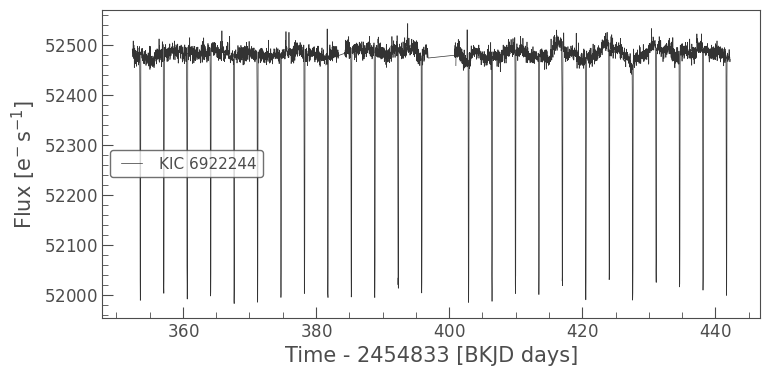
../../_images/tutorials_1-getting-started_using-light-curve-file-products_24_0.png

On this plot, the y-axis is flux in electrons per second. This unit may appear counterintutive, as flux is a measure of brightness. The CCD cameras measure an electrical charge, and so light is recorded as electrons, not photons as you might expect. On the x-axis we have time in Barycentric Kepler Julian Date (BKJD). In short, the x-axis values are days since the start of the Kepler mission. The repeating dips in brightness are transits, the effect of a planet orbiting Kepler-8 and passing between us and the star.

Note#

You can also download light curve FITS files from the archive by hand, store them on your local disk, and open them using the lk.read(<filename>) function. This function will return a KeplerLightCurve object just as in the above example. You can find out where Lightkurve stored a light curve file using the filename attribute:

[8]:

klc.filename

[8]:

'/Users/tapritc2/.lightkurve/cache/mastDownload/Kepler/kplr006922244_lc_Q111111111111111111/kplr006922244-2010078095331_llc.fits'

3. The SAP and PDCSAP Light Curves#

As you can see in the Table above, there are two different types of flux stored in the KeplerLightCurve object. These correspond to different levels of data treatment performed for this star by NASA’s Kepler Data Processing Pipeline: the simple aperture photometry (SAP) flux, and the presearch data conditioning SAP (PDCSAP) flux.

By default, a KeplerLightCurve will set the PDCSAP flux to its .flux property.

To compare the PDCSAP and the SAP flux, we can use the column keyword while plotting.

Note: alternatively, you can replace the flux column with the sap_flux column by using klc.flux = klc['sap_flux'].

[9]:

ax = klc.plot(column='pdcsap_flux', label='PDCSAP Flux', normalize=True)
klc.plot(column='sap_flux', label='SAP Flux', normalize=True, ax=ax);

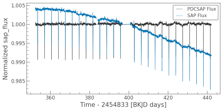
../../_images/tutorials_1-getting-started_using-light-curve-file-products_31_0.png

In brief:

The SAP light curve is calculated by summing together the brightness of pixels that fall within an aperture set by the Kepler mission. This is often referred to as the optimal aperture, but in spite of its name can sometimes be improved upon! Because the SAP light curve is a sum of the brightness in chosen pixels, it is still subject to systematic artifacts of the mission.
The PDCSAP light curve is subject to more treatment than the SAP light curve, and is specifically intended for detecting planets. The PDCSAP pipeline attempts to remove systematic artifacts while keeping planetary transits intact.

Looking at the figure we made above, you can see that the SAP light curve has a long-term change in brightness that has been removed in the PDCSAP light curve, while keeping the transits at the same depth. For most inspections, a PDCSAP light curve is what you want to use, but when looking at astronomical phenomena that aren’t planets (for example, long-term variability), the SAP flux may be preferred.

For now, let’s continue to use the PDCSAP flux only. Because this is the default .flux property of our light curve object, we don’t need to change anything.

Note#

The plot() methods in Lightkurve always return a Matplotlib object. This is useful because it lets us manipulate the plot using standard Matplotlib functions. For example, we can set the title as follows:

[10]:

ax = klc.plot()
ax.set_title("PDCSAP light curve of Kepler-8");

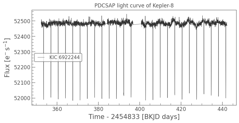
../../_images/tutorials_1-getting-started_using-light-curve-file-products_35_0.png

And the figure can be saved as follows:

[11]:

ax.figure.savefig('demo-lightcurve.png')

4. Accessing the Metadata#

When downloading data from MAST, that data usually comes in the format of a FITS file. These FITS files carry a wealth of metadata about the observation. When these are loaded in to Lightkurve to create a KeplerLightCurve, all of the metadata are stored in the .meta property of the object.

We can view these metadata by calling this property, as follows:

[12]:

klc.meta

[12]:

{'INHERIT': True,
 'EXTNAME': 'PRIMARY',
 'EXTVER': 1,
 'TELESCOP': 'Kepler',
 'INSTRUME': 'Kepler Photometer',
 'OBJECT': 'KIC 6922244',
 'KEPLERID': 6922244,
 'RADESYS': 'ICRS',
 'RA_OBJ': 281.28812,
 'DEC_OBJ': 42.45108,
 'EQUINOX': 2000.0,
 'EXPOSURE': 82.71685005,
 'TIMEREF': 'SOLARSYSTEM',
 'TASSIGN': 'SPACECRAFT',
 'TIMESYS': 'TDB',
 'BJDREFI': 2454833,
 'BJDREFF': 0.0,
 'TIMEUNIT': 'd',
 'TELAPSE': 89.84761299,
 'LIVETIME': 82.71685005,
 'TSTART': 352.36610827,
 'TSTOP': 442.21372126,
 'LC_START': 55184.87773552,
 'LC_END': 55274.70383812,
 'DEADC': 0.92063492,
 'TIMEPIXR': 0.5,
 'TIERRELA': 5.78e-07,
 'TIERABSO': <astropy.io.fits.card.Undefined at 0x17e65bd10>,
 'INT_TIME': 6.01980290327,
 'READTIME': 0.518948526144,
 'FRAMETIM': 6.538751429414,
 'NUM_FRM': 270,
 'TIMEDEL': 0.02043359821692,
 'DATE-OBS': '2009-12-19T20:49:13.619Z',
 'DATE-END': '2010-03-19T17:08:14.343Z',
 'BACKAPP': True,
 'DEADAPP': True,
 'VIGNAPP': True,
 'GAIN': 115.49,
 'READNOIS': 83.014212,
 'NREADOUT': 270,
 'TIMSLICE': 1,
 'MEANBLCK': 715,
 'LCFXDOFF': 419400,
 'SCFXDOFF': 219400,
 'CDPP3_0': 74.77433013916016,
 'CDPP6_0': 61.75667190551758,
 'CDPP12_0': 56.56961441040039,
 'CROWDSAP': 1.0,
 'FLFRCSAP': 0.8286,
 'NSPSDDET': 0,
 'NSPSDCOR': 0,
 'PDCVAR': 0.5488878488540649,
 'PDCMETHD': 'multiScaleMap',
 'NUMBAND': 3,
 'FITTYPE1': 'robust',
 'PR_GOOD1': 0.0,
 'PR_WGHT1': 0.0,
 'FITTYPE2': 'prior',
 'PR_GOOD2': 0.47542938590049744,
 'PR_WGHT2': 22.81161117553711,
 'FITTYPE3': 'prior',
 'PR_GOOD3': 0.9755752682685852,
 'PR_WGHT3': 46.809146881103516,
 'PDC_TOT': 0.45028069615364075,
 'PDC_TOTP': 0.2651563882827759,
 'PDC_COR': 0.9997496604919434,
 'PDC_CORP': 86.80510711669922,
 'PDC_VAR': 0.9991965293884277,
 'PDC_VARP': 86.88060760498047,
 'PDC_NOI': 0.9822107553482056,
 'PDC_NOIP': 99.34284210205078,
 'PDC_EPT': 1.0,
 'PDC_EPTP': 77.33592224121094,
 'CHECKSUM': '9pCbEmCZ9mCbCmCZ',
 'SIMPLE': True,
 'BITPIX': 8,
 'NAXIS': 0,
 'EXTEND': True,
 'NEXTEND': 2,
 'ORIGIN': 'NASA/Ames',
 'DATE': '2015-09-11',
 'CREATOR': '859340 FluxExporter2PipelineModule',
 'PROCVER': 'svn+ssh://murzim/repo/soc/tags/release/9.3.22 r60269',
 'FILEVER': '6.1',
 'TIMVERSN': 'OGIP/93-003',
 'CHANNEL': 31,
 'SKYGROUP': 31,
 'MODULE': 10,
 'OUTPUT': 3,
 'QUARTER': 4,
 'SEASON': 2,
 'DATA_REL': 25,
 'OBSMODE': 'long cadence',
 'MISSION': 'Kepler',
 'TTABLEID': 29,
 'PMRA': 0.0,
 'PMDEC': 0.0,
 'PMTOTAL': 0.0,
 'PARALLAX': None,
 'GLON': 71.6589,
 'GLAT': 19.012749,
 'GMAG': 13.886,
 'RMAG': 13.511,
 'IMAG': 13.424,
 'ZMAG': 13.413,
 'D51MAG': 13.7,
 'JMAG': 12.576,
 'HMAG': 12.323,
 'KMAG': 12.292,
 'KEPMAG': 13.563,
 'GRCOLOR': 0.375,
 'JKCOLOR': 0.284,
 'GKCOLOR': 1.594,
 'TEFF': 6225,
 'LOGG': 4.169,
 'FEH': -0.04,
 'EBMINUSV': 0.096,
 'AV': 0.297,
 'RADIUS': 1.451,
 'TMINDEX': 262064792,
 'SCPID': 262064792,
 'LABEL': 'KIC 6922244',
 'RA': 281.28812,
 'DEC': 42.45108,
 'FILENAME': '/Users/tapritc2/.lightkurve/cache/mastDownload/Kepler/kplr006922244_lc_Q111111111111111111/kplr006922244-2010078095331_llc.fits',
 'FLUX_ORIGIN': 'pdcsap_flux',
 'AUTHOR': 'Kepler',
 'TARGETID': 6922244,
 'QUALITY_BITMASK': 'default',
 'QUALITY_MASK': array([ True,  True, False, ...,  True,  True,  True])}

As you can see, there is a lot here if you don’t know what you are looking for! These metadata don’t just include information about the observations, but also data from the Kepler Input Catalogue (KIC) used to select observing targets, such as their magnitudes and temperature.

The .meta property is a Python dictionary, which has some convenient features. For example, we can retrieve the value of an individual keyword as follows:

[13]:

klc.meta['QUARTER']

[13]:

Alternatively, we can use the .get() method, which accounts for queries that aren’t in the dictionary.

[14]:

klc.meta.get('MISSION')

[14]:

'Kepler'

A feature of the KeplerLightCurve object is that the metadata can also be accessed via user-friendly object properties for convenience. For example, the Kepler Quarter number is directly accessible via the quarter property:

[15]:

klc.quarter

[15]:

5. Understanding the Data Arrays and Units#

As we saw above, the KeplerLightCurve object is a table that contains many arrays other than the PDCSAP and SAP fluxes. Detailed information on each of these can be found in the Kepler Archive Manual, Section 2.3.1. Light Curve Files.

The first six columns appear in all KeplerLightCurve objects, and contain the most commonly used information. These are:

time: the time measurements at each cadence.
flux: the flux of the target star at each time measurement. This is populated with PDCSAP flux by default.
flux_err: the statistical uncertainty on each flux data point.
quality: information on the data quality at each time measurement.
centroid_col & centroid_row: the position of the target star on the CCD at each observation. This changes over time due to, for example, small jitters of the spacecraft.

The remaining columns are more detailed information on the observation. Some of these are duplicated in the first five columns described above:

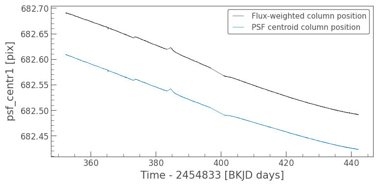
timecorr: correction values that allow users to revert back to non-barycentric timestamps.
cadenceno: these are mission-specific identifiers of each exposure.
sap_flux & sap_flux_err: the SAP flux and associated error.
sap_bkg & sap_bkg_err: the calculated background (and associated error) inside the aperture used to calculate the SAP flux.
pdcsap_flux & pdcsap_flux_err: the PDCSAP flux and associated error. Duplicated by default in flux and flux_err.
sap_quality: information on the data quality at each time measurement. Duplicated in quality.
psf_centr1 & psf_centr2 (and errors): the column and row centroid positions of a PSF model fit to the target star.
mom_centr1 & mom_centr2 (and errors): the column and row centroid positions of the target star, weighted by flux. Duplicated in centroid_col and centroid_row respectively.
pos_corr1 & pos_corr2: the column and row components of the calculated image motion.

These columns can be accessed as properties of the KeplerLightCurve , for example, as follows:

[16]:

klc.sap_bkg

[16]:

$[1672.2699,~1669.84,~1673.1306,~\dots,~1498.2946,~1498.7802,~1497.7747] \; \mathrm{\frac{e^{-}}{s}}$

The unit information of the arrays are stored using Astropy’s `astropy.units <https://docs.astropy.org/en/stable/units/>`__ module, which means that they are an Astropy `Quantity <https://docs.astropy.org/en/stable/api/astropy.units.Quantity.html#astropy.units.Quantity>`__ object. We can view the units as follows:

[17]:

print(f'Centroid column unit: {klc.centroid_col.unit}')
print(f'Flux unit: {klc.flux.unit}')

Centroid column unit: pix
Flux unit: electron / s

You can access the data in the form of a standard NumPy array using the value attribute:

[18]:

klc.centroid_col.value

[18]:

MaskedNDArray([682.69124789, 682.69084371, 682.6903808 , ...,
               682.49103683, 682.49113696, 682.49069432])

We can also plot the data using the KeplerLightCurve’s plot() method by passing a column keyword argument:

[19]:

ax = klc.plot(column='mom_centr1', label='Flux-weighted column position')
klc.plot(ax=ax, column='psf_centr1', label='PSF centroid column position');

../../_images/tutorials_1-getting-started_using-light-curve-file-products_58_0.png

Finally, the .time property is a little different. Instead of an Astropy Quantity object, it is an Astropy `Time <https://docs.astropy.org/en/stable/time/>`__ object, and has some additional time scale and format information.

[20]:

klc.time

[20]:

<Time object: scale='tdb' format='bkjd' value=[352.37632485 352.39675805 352.43762445 ... 442.16263546 442.18306983
 442.2035041 ]>

[21]:

print(f'Time scale: {klc.time.scale}')
print(f'Time format: {klc.time.format}')

Time scale: tdb
Time format: bkjd

Here, the time format is the unit of time, in this case Barycentric Kepler Julian Date (BKJD). The time scale indicates how the time is measured, in this case by taking the Barycentric Dynamical Time (TDB). This detailed information may be important when comparing observations of a periodic event (such as a planet transit) with observations made with other telescopes on Earth.

Exercises#

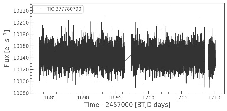
Some stars, such as Kepler-10, have been observed both with Kepler and TESS. In this exercise, download and plot the TESS PDCSAP flux only. You can do this by either selecting it from the SearchResult returned by `search_lightcurve() <https://docs.lightkurve.org/reference/api/lightkurve.search_lightcurve.html?highlight=search_lightcurve>`__ or by using the mission keyword argument when searching.

[22]:

#search_result = lk.search_lightcurvefile(...)

[23]:

# Solution:
search_result = lk.search_lightcurve('Kepler-10', mission='TESS')
search_result

[23]:

SearchResult containing 47 data products.

#	mission	year	author	exptime	target_name	distance
				s		arcsec
0	TESS Sector 14	2019	SPOC	120	377780790	0.0
1	TESS Sector 40	2021	SPOC	20	377780790	0.0
2	TESS Sector 41	2021	SPOC	20	377780790	0.0
3	TESS Sector 40	2021	SPOC	120	377780790	0.0
4	TESS Sector 41	2021	SPOC	120	377780790	0.0
5	TESS Sector 55	2022	SPOC	20	377780790	0.0
6	TESS Sector 54	2022	SPOC	20	377780790	0.0
7	TESS Sector 53	2022	SPOC	20	377780790	0.0
8	TESS Sector 55	2022	SPOC	120	377780790	0.0
9	TESS Sector 54	2022	SPOC	120	377780790	0.0
10	TESS Sector 53	2022	SPOC	120	377780790	0.0
11	TESS Sector 80	2024	SPOC	120	377780790	0.0
12	TESS Sector 81	2024	SPOC	120	377780790	0.0
13	TESS Sector 74	2024	SPOC	120	377780790	0.0
14	TESS Sector 75	2024	SPOC	120	377780790	0.0
15	TESS Sector 14	2019	TESS-SPOC	1800	377780790	0.0
16	TESS Sector 15	2019	TESS-SPOC	1800	377780790	0.0
17	TESS Sector 26	2020	TESS-SPOC	1800	377780790	0.0
18	TESS Sector 41	2021	TESS-SPOC	600	377780790	0.0
19	TESS Sector 40	2021	TESS-SPOC	600	377780790	0.0
20	TESS Sector 54	2022	TESS-SPOC	600	377780790	0.0
...	...	...	...	...	...	...
25	TESS Sector 26	2020	QLP	1800	377780790	0.0
26	TESS Sector 41	2021	QLP	600	377780790	0.0
27	TESS Sector 40	2021	QLP	600	377780790	0.0
28	TESS Sector 54	2022	QLP	600	377780790	0.0
29	TESS Sector 55	2022	QLP	600	377780790	0.0
30	TESS Sector 53	2022	QLP	600	377780790	0.0
31	TESS Sector 74	2024	QLP	200	377780790	0.0
32	TESS Sector 75	2024	QLP	200	377780790	0.0
33	TESS Sector 14	2019	TASOC	120	377780790	0.0
34	TESS Sector 15	2019	TASOC	1800	377780790	0.0
35	TESS Sector 15	2019	TASOC	1800	377780790	0.0
36	TESS Sector 14	2019	TASOC	1800	377780790	0.0
37	TESS Sector 14	2019	TASOC	1800	377780790	0.0
38	TESS Sector 15	2019	CDIPS	1800	377780790	0.0
39	TESS Sector 26	2020	TASOC	1800	377780790	0.0
40	TESS Sector 26	2020	CDIPS	1800	377780790	0.0
41	TESS Sector 26	2020	TASOC	1800	377780790	0.0
42	TESS Sector 41	2021	CDIPS	1800	377780790	0.0
43	TESS Sector 40	2021	CDIPS	1800	377780790	0.0
44	TESS Sector 55	2022	CDIPS	1800	377780790	0.0
45	TESS Sector 54	2022	CDIPS	1800	377780790	0.0
46	TESS Sector 53	2022	CDIPS	1800	377780790	0.0

Length = 47 rows

[24]:

search_result.download().plot();

/Users/tapritc2/tessgi/lightkurve_party/lightkurve/src/lightkurve/search.py:424: LightkurveWarning: Warning: 47 files available to download. Only the first file has been downloaded. Please use `download_all()` or specify additional criteria (e.g. quarter, campaign, or sector) to limit your search.
  warnings.warn(

../../_images/tutorials_1-getting-started_using-light-curve-file-products_67_1.png

About this Notebook#

Authors: Oliver Hall (oliver.hall@esa.int), Geert Barentsen

Updated On: 2020-08-31

Citing Lightkurve and Astropy#

If you use lightkurve or astropy for published research, please cite the authors. Click the buttons below to copy BibTeX entries to your clipboard.

[25]:

lk.show_citation_instructions()

[25]:

@ARTICLE{astropy:2022,
       author = {{Astropy Collaboration} and {Price-Whelan}, Adrian M. and {Lim}, Pey
       Lian and {Earl}, Nicholas and {Starkman}, Nathaniel and {Bradley}, Larry and
       {Shupe}, David L. and {Patil}, Aarya A. and {Corrales}, Lia and {Brasseur}, C.~E.
       and {N{\"o}the}, Maximilian and {Donath}, Axel and {Tollerud}, Erik and {Morris},
       Brett M. and {Ginsburg}, Adam and {Vaher}, Eero and {Weaver}, Benjamin A. and
       {Tocknell}, James and {Jamieson}, William and {van Kerkwijk}, Marten H. and
       {Robitaille}, Thomas P. and {Merry}, Bruce and {Bachetti}, Matteo and
       {G{\"u}nther}, H. Moritz and {Aldcroft}, Thomas L. and {Alvarado-Montes}, Jaime
       A. and {Archibald}, Anne M. and {B{\'o}di}, Attila and {Bapat}, Shreyas and
       {Barentsen}, Geert and {Baz{\'a}n}, Juanjo and {Biswas}, Manish and {Boquien},
       M{\'e}d{\'e}ric and {Burke}, D.~J. and {Cara}, Daria and {Cara}, Mihai and
       {Conroy}, Kyle E. and {Conseil}, Simon and {Craig}, Matthew W. and {Cross},
       Robert M. and {Cruz}, Kelle L. and {D'Eugenio}, Francesco and {Dencheva}, Nadia
       and {Devillepoix}, Hadrien A.~R. and {Dietrich}, J{\"o}rg P. and {Eigenbrot},
       Arthur Davis and {Erben}, Thomas and {Ferreira}, Leonardo and {Foreman-Mackey},
       Daniel and {Fox}, Ryan and {Freij}, Nabil and {Garg}, Suyog and {Geda}, Robel and
       {Glattly}, Lauren and {Gondhalekar}, Yash and {Gordon}, Karl D. and {Grant},
       David and {Greenfield}, Perry and {Groener}, Austen M. and {Guest}, Steve and
       {Gurovich}, Sebastian and {Handberg}, Rasmus and {Hart}, Akeem and
       {Hatfield-Dodds}, Zac and {Homeier}, Derek and {Hosseinzadeh}, Griffin and
       {Jenness}, Tim and {Jones}, Craig K. and {Joseph}, Prajwel and {Kalmbach}, J.
       Bryce and {Karamehmetoglu}, Emir and {Ka{\l}uszy{\'n}ski}, Miko{\l}aj and
       {Kelley}, Michael S.~P. and {Kern}, Nicholas and {Kerzendorf}, Wolfgang E. and
       {Koch}, Eric W. and {Kulumani}, Shankar and {Lee}, Antony and {Ly}, Chun and
       {Ma}, Zhiyuan and {MacBride}, Conor and {Maljaars}, Jakob M. and {Muna}, Demitri
       and {Murphy}, N.~A. and {Norman}, Henrik and {O'Steen}, Richard and {Oman}, Kyle
       A. and {Pacifici}, Camilla and {Pascual}, Sergio and {Pascual-Granado}, J. and
       {Patil}, Rohit R. and {Perren}, Gabriel I. and {Pickering}, Timothy E. and
       {Rastogi}, Tanuj and {Roulston}, Benjamin R. and {Ryan}, Daniel F. and {Rykoff},
       Eli S. and {Sabater}, Jose and {Sakurikar}, Parikshit and {Salgado}, Jes{\'u}s
       and {Sanghi}, Aniket and {Saunders}, Nicholas and {Savchenko}, Volodymyr and
       {Schwardt}, Ludwig and {Seifert-Eckert}, Michael and {Shih}, Albert Y. and
       {Jain}, Anany Shrey and {Shukla}, Gyanendra and {Sick}, Jonathan and {Simpson},
       Chris and {Singanamalla}, Sudheesh and {Singer}, Leo P. and {Singhal}, Jaladh and
       {Sinha}, Manodeep and {Sip{\H{o}}cz}, Brigitta M. and {Spitler}, Lee R. and
       {Stansby}, David and {Streicher}, Ole and {{\v{S}}umak}, Jani and {Swinbank},
       John D. and {Taranu}, Dan S. and {Tewary}, Nikita and {Tremblay}, Grant R. and
       {Val-Borro}, Miguel de and {Van Kooten}, Samuel J. and {Vasovi{\'c}}, Zlatan and
       {Verma}, Shresth and {de Miranda Cardoso}, Jos{\'e} Vin{\'\i}cius and {Williams},
       Peter K.~G. and {Wilson}, Tom J. and {Winkel}, Benjamin and {Wood-Vasey}, W.~M.
       and {Xue}, Rui and {Yoachim}, Peter and {Zhang}, Chen and {Zonca}, Andrea and
       {Astropy Project Contributors}}, title = "{The Astropy Project: Sustaining and
       Growing a Community-oriented Open-source Project and the Latest Major Release
       (v5.0) of the Core Package}",
      journal = {\apj},
     keywords = {Astronomy software, Open source software, Astronomy data analysis, 1855, 1866, 1858, Astrophysics - Instrumentation and Methods for Astrophysics},
         year = 2022,
        month = aug,
       volume = {935},
       number = {2},
          eid = {167},
        pages = {167},
          doi = {10.3847/1538-4357/ac7c74},
archivePrefix = {arXiv},
       eprint = {2206.14220},
 primaryClass = {astro-ph.IM},
       adsurl = {https://ui.adsabs.harvard.edu/abs/2022ApJ...935..167A},
      adsnote = {Provided by the SAO/NASA Astrophysics Data System}
}

@ARTICLE{2019AJ....157...98G,
   author = {{Ginsburg}, A. and {Sip{\H o}cz}, B.~M. and {Brasseur}, C.~E. and
    {Cowperthwaite}, P.~S. and {Craig}, M.~W. and {Deil}, C. and
    {Guillochon}, J. and {Guzman}, G. and {Liedtke}, S. and {Lian Lim}, P. and
    {Lockhart}, K.~E. and {Mommert}, M. and {Morris}, B.~M. and
    {Norman}, H. and {Parikh}, M. and {Persson}, M.~V. and {Robitaille}, T.~P. and
    {Segovia}, J.-C. and {Singer}, L.~P. and {Tollerud}, E.~J. and
    {de Val-Borro}, M. and {Valtchanov}, I. and {Woillez}, J. and
    {The Astroquery collaboration} and {a subset of the astropy collaboration}
    },
    title = "{astroquery: An Astronomical Web-querying Package in Python}",
  journal = {\aj},
archivePrefix = "arXiv",
   eprint = {1901.04520},
 primaryClass = "astro-ph.IM",
 keywords = {astronomical databases: miscellaneous, virtual observatory tools},
     year = 2019,
    month = mar,
   volume = 157,
      eid = {98},
    pages = {98},
      doi = {10.3847/1538-3881/aafc33},
   adsurl = {http://adsabs.harvard.edu/abs/2019AJ....157...98G},
  adsnote = {Provided by the SAO/NASA Astrophysics Data System}
}

When using Lightkurve, we kindly request that you cite the following packages:

lightkurve
astropy
astroquery — if you are using search_lightcurve() or search_targetpixelfile().
tesscut — if you are using search_tesscut().

Space Telescope Logo

Searching & downloading Kepler, K2, and TESS data

Using Target Pixel Files with Lightkurve

Using Light Curve Files with Lightkurve#

Learning Goals#

Introduction#

Imports#

1. About NASA’s Photometric Space Telescopes#

1.1. Kepler#

1.2. K2#

1.3. TESS#

2. Downloading a Light Curve File#

Note#

3. The SAP and PDCSAP Light Curves#

Note#

4. Accessing the Metadata#

5. Understanding the Data Arrays and Units#

Exercises#

About this Notebook#

Citing Lightkurve and Astropy#

1.1. Kepler #

1.2. K2 #

1.3. TESS #